Search the data

User guide to the GEBCO One Minute Grid

Contents

1. Introduction
2. Developers of regional grids
3. Gridding methods
4. Assessing the quality of the grid
5. Limitations of the GEBCO grid
6. Format and compatibility of the grid
7. How to give feedback and become involved with GEBCO

Appendix A — Review of the problems of generating a gridded data set from the GEBCO Digital Atlas contours

1. The uses of and requirements for gridded bathymetry data
2. History of gridded bathymetry and GEBCO's interest in it
3. Mathematical representations of bathymetry, contours, and grids
4. The representation of bathymetry in the GEBCO contours
5. Preparing grids from contours (and possibly other information)
6. References

Appendix B — Version 2.0 of the GEBCO One Minute Grid (November 2008)

Originally released in 2003, this document has been updated to include information about version 2.0 of the GEBCO One Minute Grid, released in November 2008.

Acknowledgements

This document was prepared by Andrew Goodwillie (Formerly of Scripps Institution of Oceanography) in collaboration with other members of the informal Gridding Working Group of the GEBCO Sub-Committee on Digital Bathymetry (now called the Technical Sub-Committee on Ocean Mapping (TSCOM)).

Generation of the grid was co-ordinated by Michael Carron with major input provided by the gridding efforts of Bill Rankin and Lois Varnado at the US Naval Oceanographic Office, Andrew Goodwillie and Peter Hunter. Significant regional contributions were also provided by Martin Jakobsson (University of Stockholm), Ron Macnab (Geological Survey of Canada (retired)), Hans-Werner Schenke (Alfred Wegener Institute for Polar and Marine Research), John Hall (Geological Survey of Israel (retired)) and Ian Wright (formerly of the New Zealand National Institute of Water and Atmospheric Research). Technical advice and support on algorithms was provided by Walter Smith of the NOAA Laboratory for Satellite Altimetry.

Back to top

1.0 Introduction

1.1 Definition and advantages of a grid

A grid is a computer based representation of a three-dimensional ( x,y,z ) data set. In a gridded database, the z value is given at equidistantly spaced intervals of x and y . In our case, the GEBCO bathymetric grid, the z value is the depth to the sea floor and is given at evenly spaced increments of longitude ( x ) and latitude ( y ).

Gridded databases are ideally suited for computer-based calculations. In binary form, they are compact and permit subsets of the data to be easily extracted. They allow comparison with other gridded databases, and facilitate the plotting, visualisation and ready analysis of the grid values.

1.2 GEBCO recognition for gridded bathymetry

Bathymetry represents a fundamental measure of Earth's physiography. Although climate modellers, oceanographers, geologists, and geophysicists consider bathymetry to be a key parameter in their fields, the world's oceanic areas remain poorly mapped overall. Indeed, the surfaces of the moon, Mars, Venus and numerous planetary satellites are better surveyed than the ocean floor. That said, GEBCO aims to provide the most accurate global bathymetry data set derived from echo soundings that is publically available.

Ten years ago, GEBCO bathymetry was available in one form only ie. as hard copy printed map sheets. Although a generation of earth scientists had grown familiar with this series of 18 GEBCO portrayals covering the entire globe, the use of paper charts was becoming restrictive. In 1994, GEBCO released on CDROM a digitized version of its standard 500m interval contours. This CDROM, called the GEBCO Digital Atlas (GDA) contained data files of digitised contours, a software interface for PC, and a detailed documentation booklet.

The GDA represented the culmination of a decade's work by numerous individuals and institutions around the globe, and the shift from paper charts to digitised contours made the GEBCO contour data set more versatile. However, by the early 1990s, the increasing availability of low cost, powerful computers meant that the use of gridded databases was becoming widespread. Digitised contours alone did not offer the advantages of a three-dimensional grid.

At its 1994 annual meeting, the volunteers that comprise the membership of GEBCO's Sub-Committee on Digital Bathymetry (SCDB) recognised the widely expressed need of earth scientists for a high quality gridded depth database, and agreed to explore the construction of a gridded version of GEBCO bathymetry, at a grid spacing of 5 arc minutes. An SCDB Grid Working Group was initiated.

At the 1997 GEBCO SCDB meeting, it was agreed that construction of the GEBCO global grid would use as input the latest available GDA digitised contours and that the resultant grid depths would match these GDA contours as closely as possible. Members of the grid working group were assigned the responsibility of producing particular regional grids. When combined, these regional grids would constitute GEBCO's global bathymetric grid with 100% coverage of the world's oceanic areas.

In 1998, at the next SCDB meeting, it was decided that the grid would contain both sea floor bathymetry and land topography — it would be a continuous digital terrain model. Also at that meeting, the resolution specification of the grid was increased to a spacing of 2.5 arc minutes which would make it comparable in resolution to other earth science global databases. At a subsequent GEBCO meeting, this resolution was increased still further, to a one minute grid spacing.

The construction of a gridded depth database from digitised contours posed a number of non-trivial problems and it was early recognised by members of the SCDB Grid Working Group that one method alone could not be used to construct the entire global grid. Evolving technical developments and gridding techniques would result in each regional grid having a unique character that would reflect the style of contouring, the method of grid construction, and location of region. However, the edge match between adjacent regional grids would be seamless.

The minutes from recent GEBCO meetings provide a detailed summary of the development of the GEBCO one minute bathymetric grid. These minutes can be found on GEBCO's web site http://www.gebco.net/about_us/meetings_and_minutes/

Back to top

2.0 Developers of regional grids

The formidable task surrounding the compilation of source echo soundings and their subsequent interpretation by bathymetrists to produce the GEBCO GDA contours is described fully in the GDA documentation. Like the compilation of those GDA contours, the construction of the GEBCO one minute global bathymetric grid has almost exclusively been the result of a purely voluntary effort by a number of scientists and institutions around the globe.

Shown in Figure 1 are the regional grids that comprise the GEBCO global one minute bathymetric grid. The GEBCO member or group responsible for creating each of these grids is listed below. Input data sources — soundings and contours — that were used in addition to the main GDA contours are also given.

Digitisation of the GDA contours, track lines, and coastline data was performed by Pauline Weatherall at the British Oceanographic Data Centre (BODC). Supplemental digitisation was provided by the organisations referenced in the User Guide to the GDA Data Sets.

Edge matching and the editing of GDA contours along common grid boundaries were performed by Pauline Weatherall (BODC).

The current contact details of GEBCO members can be found on GEBCO's web page at http://www.gebco.net/about_us/contact_us/

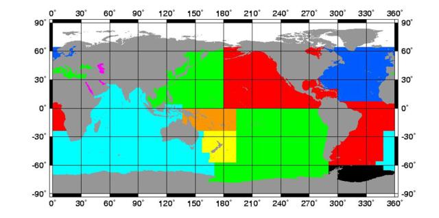
Figure 1. The main regional grids of the GEBCO one minute global grid are identified by section number as follows. Light blue - 2.1. White - 2.2. Red - 2.3. Green - 2.4. Black - 2.5. Dark blue- 2.6/2.11. Fuchsia - 2.7. Orange - 2.8. Yellow - 2.9.,

2.1 Indian Ocean and Environs

Andrew Goodwillie — from the extensive new bathymetric data compilation and contour interpretation by Robert Fisher. The grid includes additional intermediate level contours in abyssal plains and the Bay of Bengal, and South African shallow water shelf contours.

2.2 Arctic Ocean (64° N to North Pole)

Martin Jakobsson and Ron Macnab — from the IBCAO (Arctic Ocean) compilation v1. http://www.ngdc.noaa.gov/mgg/bathymetry/arctic/

2.3 South Atlantic, NE Pacific, Gulf of Mexico, portions of N Atlantic, Hudson Bay

William Rankin — Includes data from the IBCCA (Caribbean and Gulf of Mexico) compilation, and from Germany, UK and USA. http://www.ngdc.noaa.gov/mgg/ibcca/ibcca.html

2.4 NW Pacific, SE Pacific, Mediterranean Sea, Black Sea

Michael Carron — includes Japanese shelf data and additional US data.

2.5 Weddell Sea

Hans-Werner Schenke — largely from original Antarctic bathymetric data collected by Alfred-Wegener-Institut fur Polar-und Meeresforschung.

2.6 North Atlantic (large portions)

Peter Hunter and Ron Macnab — Includes data supplied by Canada, France, UK and USA.

2.7 Red Sea, Caspian Sea, Persian Gulf

John Hall — includes IBCM data and major data contributions from Russia, France, Israel. http://www.ngdc.noaa.gov/mgg/ibcm/ibcm.html

2.8 Equatorial Western Pacific

Lois C. Varnado.

2.9 New Zealand waters

National Institute of Water and Atmospheric Research, New Zealand. http://www.niwa.cri.nz/

2.10 USA Continental Shelf

High resolution bathymetric grid provided by National Geophysical Data Center, Boulder. http://www.ngdc.noaa.gov/mgg/coastal/coastal.html

2.11 Baltic Sea

Torsten Seifert — Institut fur Ostseeforschung Warnemuende, Germany.

2.12 Japan region, shallow water

Japan Meteorological Office. From Japan Hydrographic Office data.

Back to top

3.0 Gridding method

Below, is summarised the general methodology that was used for the construction of most of the GEBCO regional grids. This summary is intended to be an overview to the gridding process. It does not cover the techniques that were used by all GEBCO gridders.

Refer to the individual GEBCO gridders listed in section 2.0 and to the references therein for specific information on gridding techniques.

GEBCO gridders made much use of the Wessel and Smith GMT software for construction and quality control of the grids ( http://gmt.soest.hawaii.edu/ ).

Each regional grid was divided into smaller subgrids, generally of 10°x10°. This had the advantage of rapid computation of the interpolated bathymetric grid values and of facilitating the task of error checking the resultant grid depths.

In constructing each 10°x10° sub-grid an additional border of 5° was added. This 5° overlap helped to maintain the continuity and smoothness of the grid surface such that step function depth discontinuities along common edges were minimised when adjacent 10°x10° sub-grids were joined together.

3.1 Accumulation of input data

One input data file, in (longitude, latitude, depth) format, is created. It contains

• Digitised current GEBCO GDA contours
• GLOBE land elevations
• WVS coastlines
• SCAR (Antarctic) coastlines
• Additional shallow water contours and soundings
• Additional intermediate contours in featureless areas
• Additional individual echo soundings

3.2 Decimation of input data

Divide the area of the subgrid into 1x1 arc minute bins — use a median filter ( GMT: blockmedian ) or mean filter ( GMT: blockmean ) to thin the data points within each 1x1 minute bin. This acts to reduce the effect of erratic input data and it speeds up the grid computation. Note that, at this decimation stage, bins that contain no input data points remain empty.

GMT command example, for the sub-grid bounded by 150° - 160° E/20° - 30° S:

% blockmedian input_data.xyz -R145/165/-35/-15 -I1m -V > input_data.bm

3.3 Compute a 3D gridded surface

The 1x1 minute thinned data file is fed into a surface fitting computer program ( GMT: surface ) which uses as its interpolation algorithm a 3D bicubic spline under tension. This program computes a depth value at each grid node. By this process of interpolation each 1x1 minute bin in the 10°x10° subgrid is now associated with an interpolated depth value.

GMT command example:

% surface input_data.bm -R145/165/-35/-15 -I1m -C1 -T0.35 -V -Gtemp.grd
% grdcut temp.grd -R150/160/-30/-20 -V -Ggrid_150e_160e_30s_20s.grd

3.4 Compare grid depths to the input GDA contours

Recall from section 1.2 that the prime requirement of the GEBCO gridded bathymetry is that it matches — as closely as possible — the input GDA contours. Forcing a rigorous 3D mathematical grid model to fit the interpreted geological characteristics that are built into the GDA contours can never result in a perfect match. These mismatches are present as artefacts in the resultant grid.

The most convenient way of comparing the grid depths and input depths is found to be by visual means. Plots made in a Mercator projection at a scale of four inches to one degree (about 1:1,000,000 at the equator) allow even the smallest of artefacts to be investigated, as follows.

The gridded bathymetry is plotted in plan view as a coloured surface. It is overlain by the digitised input GDA contours. With colour palette changes specified at the same depths as the input GDA contours any colour change that is not bounded by a GDA contour is considered to be an artefact. This simple visual technique allows gross gridding mismatches to be readily seen. The use of artificial illumination on these plots reveals more subtle grid artefacts many of which lie within one colour palette band.

3.5 Main types of grid errors

The most common grid artefacts were overshoots in areas of relatively steep topography. The 500 m standard GEBCO contour interval and the overall lack of shallow water data caused many overshoots at the tops and bases of continental shelves, seamount summits, ridges, rises and plateaux. (See Figure 5.1 in Appendix A for an example of an overshoot.)

Another common artefact, due to the general absence of finer interval contours in relatively featureless abyssal plains, sediment fans, basins and wide continental shelves, produced extensive areas of erroneous depths.

In some regions, an unexpected source of gridding error came from GDA contours that had been digitised at a relatively sparse along contour sampling interval.

More minor artefacts were produced by mislabelled GDA contours and by some unreliable echo soundings that were used as additional input.

3.6 Minimisation of grid artefacts

1. Adjustment of the grid surface tension factor (see section 3.3) could reduce the overshoots but could also produce mismatches elsewhere in the grid. For consistency each gridder used one tension factor within their grids. A tension factor of 0.35 was found to be appropriate for a wide range of bathymetric features.
2. Ideally, a grid is produced by the gridding of at least one data point per bin. In the case of the GEBCO global bathymetric grid, there are many 1x1 minute bins that are devoid of digitised GDA contour input data.
   In areas of widely-spaced contours such as abyssal plains and wide continental shelves it was essential to help constrain the grid calculation through the addition of echo-soundings and intermediate-level contours. Gridders reverted, where possible, to the original data compilation sheets created by the bathymetrists. Even so, the effort required to meticulously compile additional constraining data was large, particularly the drawing and digitization of intermediate-level contours and the manual key-entering of individual reliable echo-sounding depths.
   After these additional constraining points are added to the input data file (step 3.1), steps 3.2 - 3.4 are repeated until all gridding artefacts are minimised.
3. Once GEBCO gridders gained insight into the nuances of their gridding procedures, it was possible to pre-emptively address portions of the grid that had a high potential for otherwise producing grid artefacts — before making the grid, extra depth values in these flagged areas were added to the input data file. This greatly reduced the number of iterations that needed to be performed before a grid was considered finished.

3.7 Antarctic coastlines

In the Indian Ocean, Antarctic (SCAR) coastlines with SCAR codes of 22010 - 22023 were considered to be permanent ice or other permanent coastline. They were taken to have a depth of zero metres. Depths beneath permanent ice were not determined.

Floating and seasonal ice edges (SCAR coastlines coded 22030 - 22050) were excluded from the gridding process. In these locations, the underlying sea floor was modelled by surface from surrounding bathymetry and permanent coastlines.

3.8 Main exceptions to general gridding methodology

1. The Arctic Ocean grid was constructed on a polar stereographic projection. And, its primary source of bathymetric data is from previously unavailable digital echo soundings and contours.
2. GDA contours in the S Atlantic, NW and SE Pacific are only sparsely sampled in the along contour direction. For these areas it was necessary to interpolate more digitised points along contour in order to ensure the presence of at least one digitised contour point for every arc minute of contour length.
3. Grids for the S Atlantic, NW and SE Pacific did not use land elevations in the original input data. Instead, after the bathymetric grid had been accepted, grid values above sea level were replaced with GLOBE values.
4. Grids for the Red Sea, Caspian Sea, and Persian Gulf were constructed at a spacing of 0.1 minutes and then degraded to one minute for inclusion in the GEBCO global grid.
5. The high resolution US Continental Shelf Coastal Relief Model was degraded to one minute for inclusion in the GEBCO global bathymetric grid.

3.9 Related web links and references

Land elevations — GLOBE (v2) — http://www.ngdc.noaa.gov/mgg/topo/globe.html
US Coastal Relief Model — http://www.ngdc.noaa.gov/mgg/coastal/coastal.html
SCAR (v3) coastlines — http://www.add.scar.org/
WVS coastline (NIMA) — http://www.add.scar.org/
GMT software — http://gmt.soest.hawaii.edu/

Jakobsson, M., Cherkis, N., Woodward, J., Coakley, B., and Macnab, R., 2000, A new grid of Arctic bathymetry: A significant resource for scientists and mapmakers, EOS Transactions, American Geophysical Union, v. 81, no. 9, p. 89.

Goodwillie, A. M., 1996. Producing Gridded Databases Directly From Contour Maps. University of California, San Diego, Scripps Institution of Oceanography, La Jolla, CA. SIO Reference Series No. 96-17, 33p.

Back to top

4.0 Assessing the quality of the grid

The prime goal in the construction of the GEBCO one minute global bathymetric grid was to match — as closely as possible — the input GDA contours. A grid that replicates the input depths exhibits no difference between the mathematically modelled grid depths and the input depths. Any non-zero differences indicate mismatches introduced by the 3D surface fitting process.

To quantify these differences one can extract ( GMT: grdtrack ) grid depths at the same locations as the input digitised GDA contours (and at any additional non-GDA contours and soundings). Differencing the grid and input depth values gives a measure of the closeness of fit of the gridded surface. As an example, the 10°x10° subgrids in the Indian Ocean typically yield 95% of grid depth values within 50m of the input depth values. In areas generally devoid of GDA contours such as extensive abyssal plains, this differencing method will allow us to quantify the closeness of fit only if additional input contours and soundings were used there.

Assessing grid quality simply as a difference between grid and input depths fails to take into account the wealth of data and expert geological knowledge that were used by the bathymetrists to painstakingly construct the GDA contours. Each bathymetrist used their own unique set of criteria to produce these contours. Thus, some measure of the quality of the contouring is perhaps more useful than a statistic determined from the grid depths. However, the subjective and interpretative nature of these GDA contours makes even their assessment difficult.

One approach to deriving a measure of contour quality is to create geographic plots showing the distribution of the raw data used to derive the bathymetric GDA contours — shipboard echo soundings lines and any additional soundings. This allows us to judge the reliability of the GDA contours. Care must be taken over the type of map projection chosen to ensure a balanced view of track line density. A track plot, however, does not take into account the large number of additional contours from numerous sources that were used in the derivation of GDA contours and of the grid. And, it could include portions of digitised track lines for which the bathymetrist had deemed the soundings unreliable.

Alternatively, a geographic plot showing the distribution of all digitised data that were used as input to the gridding process — GDA contours, additional non-GDA contours, individual additional echo soundings, and any along track soundings — would accurately show their areal coverage. This provides a measure of the distance of a grid point to the nearest input (constraining) data point but tells us nothing of the accuracy of the grid depths.

In summary, attempting to impose an all encompassing numerical quality factor — whether statistically determined or otherwise — upon the grid and upon the subjectively derived GDA contours is not straightforward. The difficulty in producing grids from disparate data sources and in assessing their quality is discussed extensively in Appendix A. Contact the gridder listed in section 2 for specific details of how the quality of their grids was measured.

Back to top

5.0 Limitations of the GEBCO grid

1. GEBCO, traditionally, has concentrated upon the interpretation of bathymetry in deep water. For decades, its standard contours have been fixed at intervals of 500 m (500 m, 1000 m, 1500 m, 2000 m, etc.) with a 200 m and 100 m contour in shallow zones only where justified. Although significant quantities of bathymetry data contoured at intervals of 200 m and even 100 m have been incorporated into GEBCO bathymetry, the standard 500 m contours comprise the bulk of the current GEBCO GDA contour data set. Their style and character is unique, reflecting the interpretative skill and experience of each of the GEBCO contourers. Plotting the grid depths as a histogram reveals numerous peaks each of which occurs at a multiple of 500 m. These peaks correspond to the 500 m contour interval of the input digitised GDA contour data. This terracing effect is a well known problem of constructing grids from contours.
2. It is conceivable that a bathymetric feature of up to 500 m in height would be excluded from the GDA contours if its base and peak fall just inside a 500 m level contour. However, by careful examination of the source echo soundings data the bathymetrists strove to avoid this scenario by ensuring that there was some indication in the resultant bathymetric contours of the presence of such a feature.
3. The standard GEBCO contour interval is 500 m. In some locations, additional intermediate contours (at the 200 m or 100 m interval) were used to constrain the grid calculation. And, on some continental shelves, very shallow contours were input. Compared to total coverage, high resolution multibeam bathymetric surveys it will likely prove unjustifiable to plot the GEBCO global grid at a fine contour interval of, say, 10 m or 20 m except in very rare cases (where contours of this interval size were used as input).
4. The 1x1 minute bin size used in the GEBCO global bathymetric grid does not imply that input data were this densely distributed. See section 4.0. Even after the inclusion of much additional constraining contours and soundings data, many 1x1 minute bins remained unpopulated.
5. The 1x1 minute bins become thinned in the E - W direction away from the equator which results in non-uniform grid interpolation. This latitude dependent distortion of bin geometry required that the Arctic Ocean grid be constructed using a specialised method (see section 2). Except for the Arctic Ocean this distortion was considered an acceptable compromise of the generalised gridding method described in
   section 3. Assuming a spherical earth, the 1x1 minute bin dimensions vary with latitude as follows:

   Latitude (N or S)	Bin width (E - W)	Bin height (N - S)
   0°	1.85 km	1.85 km
   30°	1.60 km	1.85 km
   45°	1.31 km	1.85 km
   60°	0.92 km	1.85 km
   72°	0.57 km	1.85 km

6. Due to the size of the geographical areas gridded and to the number of grid artefacts found, only grid mismatches of more than a few kilometres in size were investigated and eliminated or reduced.
7. No thorough error checking was performed for land areas. The very high density of GLOBE land elevation data was taken as accurate.
8. The grid is not intended to be used for navigational purposes.

Back to top

6.0 Format and compatibility of the grid

GEBCO's gridded data sets are made available in netCDF, in the form of both two-dimensional (2D) and one-dimensional (1D) arrays of signed 2-byte integers. In addition, the 2D gridded data set uses the NetCDF Climate and Forecast (CF) Metadata Convention ( http://cf-pcmdi.llnl.gov/ ).

The 1D grid file format is aimed specifically for use with the GEBCO Digital Atlas software interface and GEBCO Grid Display software. Please note that these software packages will not work with the 2D grid format files but solely with the global 1D grid files.

Information concerning netCDF format can be found at — http://www.unidata.ucar.edu/packages/netcdf/

2D CF-netCDF format

Within the 2D CF-netCDF file, the grid is stored as a two-dimensional array of 2-byte signed integer values of elevation in metres, with negative values for bathymetric depths and positive values for topographic heights.

The complete data set gives global coverage, spanning 90° N, 180° W to 90° S, 180° E on a one arc-minute grid. The grid consists of 10,801 rows x 21,601 columns giving a total of 233,312,401 points. The data values are grid line registered i.e. they refer to elevations centred on the intersection of the grid lines.

The data file includes header information which conforms to the NetCDF Climate and Forecast (CF) Metadata Convention ( http://cf-pcmdi.llnl.gov/ ).

Please note that 2D grid format files will not work with either the GEBCO Digital Atlas software interface or the GEBCO Grid Display software package — these packages are designed to use the 1D version of GEBCO's grids.

1D netCDF format

Within the 1D netCDF file, the grid is stored as a one-dimensional array of 2-byte signed integer values of elevation in metres, with negative values for bathymetric depths and positive values for topographic heights.

The complete data set gives global coverage. Each consists of 10,801 rows x 21,601 columns, resulting in a total of 233,312,401 points. The data start at position 90° N, 180° W and are arranged in latitudinal bands of 360 degrees x 60 points per degree + 1 = 21,601 values. The data range eastward from 180° W to 180° E. i.e. the 180° value is repeated. Thus, the first band contains 21,601 repeated values for 90° N, then followed by a band of 21,601 values at 89° 59' N and so on at one minute latitude intervals down to 90° S. The data values are pixel centre registered i.e. they refer to elevations at the centre of grid cells.

This grid file format is suitable for use with the GEBCO Digital Atlas Software Interface and GEBCO Grid display software.

Please note that for ease of import into Esri ArcGIS Desktop software packages it is suggested that the 2D versions of GEBCO's grids are used. However, through the GridViewer and GDA software interfaces the data can be exported in an ASCII form suitable for conversion to an Esri raster.

Back to top

7.0 How to give feedback and become involved with GEBCO

We need your feedback! If you have detected any problems in GEBCO's global bathymetric grids, vector data sets, the software interface or in this documentation please let us know. You can contact GEBCO via the "Contact us" button on GEBCO's home web page — http://www.ngdc.noaa.gov/mgg/gebco/gebco.html

GEBCO is a largely voluntary group of individuals and organisations that share a common vision — the provision of the best available bathymetry for the world's oceans. As a scientific association we welcome your ideas and suggestions and we invite you to become an active member of GEBCO.

Of course, if you are willing to contribute any bathymetric data sets (cruise files, data compilations, soundings sheets, and so on) that are not already part of the GEBCO bathymetric compilation this would be greatly appreciated. All contributions will be fully accredited and acknowledged.

Back to top

APPENDIX A — Review of the problems of generating a gridded data set from the GEBCO Digital Atlas contours

In 1994, an informal Working Group /Task Team was set up by the GEBCO Sub-Committee on Digital Bathymetry to explore the issues that might be involved in generating a gridded version of GEBCO.

The group was led by Walter Smith of the US National Ocean Survey (now at the NOAA Laboratory for Satellite Altimetry) and, in 1997, it produced a draft document entitled 'On the preparation of a gridded data set from the GEBCO Digital Atlas contours'. The document provides a useful review of the problems of gridding and is reproduced here as background to the thinking behind the generation of the GEBCO One Minute Grid.

On the preparation of a gridded data set from the GEBCO Digital Atlas contours

By the task group on gridding of the GEBCO SCDB
Version 9 - 16 June 1997

Summary

A gridded data set, simply called a grid, is one in which estimates of a quantity are given at locations equidistantly spaced along two co-ordinates, such as latitude and longitude. This regular spacing greatly facilitates machine based computations and therefore gridded bathymetry is used in a wide variety of applications. Section 1 anticipates the needs of various users of gridded bathymetry. By keeping these needs in mind, GEBCO may be able to design a particularly useful product. Section 2 reviews the history of gridded bathymetry and GEBCO's efforts leading to this report. Section 3 describes contours and grids from the mathematical point of view. Section 4 uses contours from the GEBCO Digital Atlas 1997 (the "GDA") to illustrate that GDA contours have interpretive geological value which is not easily described mathematically or captured by a machine algorithm. Section 5 briefly outlines methods for estimating grid values ("gridding algorithms") from contours and from spot depths, describing the strengths and weaknesses of various methods and the compromises which must be made in selecting one.

Back to top

A.1. The uses of and requirements for gridded bathymetry data

A.1.1 General use and visualisation

Grids are generally useful because the presence of data at regularly spaced locations facilitates many kinds of calculations, and because most computer display devices (printers, monitors, and other video and film writers) have a grid of display co-ordinates (pixels). Transformation of data from one map projection to another, and expansion in basis functions such as splines, Fourier series, and spherical harmonics are all easily done with gridded data and are much more difficult with other kinds of data. A global grid will have locations on land as well as in the ocean, and will be most easily used if some estimate of land elevations is included in addition to the GEBCO bathymetry.

Computer visualisation methods including perspective views and "shading" or "artificial illumination" of data sets are also common and helpful techniques of data interpretation and illustration which require gridded data. They are not very successful, however, unless the first differences of the gridded data (the numerical approximation of the first derivatives of the data in the grid directions) are also fairly reliable. This is because these techniques involve calculating the angle of the local perpendicular to the gridded bathymetric surface. Most of the gridding algorithms which are specialised to grid contour data yield a grid with poor quality derivatives, unfortunately. Better derivatives can be obtained from a "higher order" method (described below) but at the expense of possible violations of other desirable constraints.

A.1.2 Specific needs of physical oceanography

The Scientific Committee on Oceanic Research (SCOR) has convened a Working Group on Improved Global Bathymetry (SCOR WG 107) to assess the need for bathymetric data in research problems in physical oceanography. Preliminary investigations suggest that small changes in bathymetry in local areas can have large effects on the calculated estimates of tidal amplitudes and phases throughout an ocean basin. The sensitivity of computer models of global ocean circulation to changes in bathymetry is also under investigation. It appears that computational power and understanding of fluid dynamics have advanced to the point that bathymetry may soon be the limiting factor in modeling ocean dynamics.
Computer models which simulate the general ocean circulation solve the hydrodynamical equations at a network of points described as a set of fixed depths at each point in a horizontal grid. This strategy takes advantage of the fact that forcings and flows are dominantly horizontal, and so the stratification of the model achieves a computational simplification. Therefore these modelers need to be able to determine at what grid locations a given horizontal layer is connected or isolated. That is, which grid points comprise a basin which is closed below a given layer depth, and where are there troughs which allow deep water flow between basins? Accurate modeling of the deep water flow is important to long-term forecasts of climate change. Therefore, an ocean circulation modeler might want a grid which specifies the deepest level that is encountered in an area, or which facilitates the calculation of the deepest level at which water can flow horizontally.

In sufficiently shallow water, tides are influenced by frictional interaction with the sea bottom. While the bathymetric needs of tide modelers have not been clearly stated yet, it is possible that at some time in the near future the tide modelers might need a grid which facilitates calculation of the roughness of the bottom, or the sediment type of the bottom, from the morphological characteristics of the bathymetric grid. The roughness calculation might require accurate horizontal derivatives in the grid, or it might be useful to have a grid of the standard deviations of depths in a grid cell, or the extrema (shallowest and deepest points) of each cell. In addition, seamounts that protrude into the thermocline contribute to tidal dissipation. Recently available satellite altimeter data have revealed that seamounts are more numerous in some areas than previous charts showed. If gridded bathymetry are used to estimate the tidal dissipation caused by seamounts, then the grid should accurately portray the number and locations of seamounts and their summit depths.

A.1.3 Specific needs of marine geophysics

All of the above properties are useful in geophysical applications. The recent literature on estimation of thermal properties of the oceanic lithosphere and mantle makes clear that some geophysicists will take a grid of bathymetry and try to fit models to it by statistical regression. In this case it is important that the geophysicist should be able to guess the likely error of the depth estimate at each grid point, if an explicit estimate is not supplied with the gridded data. (The uncertainty might depend on the variability of depth in the region and the distance to the nearest control data.) The statistical regression procedure supposes that depths which are erroneously deep are as likely as depths which are erroneously shallow. The error distribution of actual bathymetric data is unlikely to have this property — on the one hand, hydrographers often are concerned to report the shallowest depth in a region — on the other hand, many shallowing features such as seamounts may have escaped detection.

Grids which have the statistical problem known as "terracing" are particularly unsuited to regression analysis. Terracing is an artifact of the gridding of contours by some gridding algorithms. It refers to a situation in which the grid contains depth values close to the values of the control contours much more frequently than it contains other values. Thus the gridded surface seems to represent a surface which does not slope smoothly between contours, but steps between nearly flat terraces at contour levels. In this case the geophysicist's statistical assumption that the depths are smoothly distributed will be severely violated, leading to biased estimates of geophysical parameters (Smith, 1993).

A.1.4 Properties of the ideal grid

Ideally, a grid would be

1. a faithful representation of depth in the ocean
2. with no gaps on land
3. having first derivatives which are suitable for visualisation techniques
4. free of statistical anomalies and other biases such as "terracing"
5. accompanied by quality and ancillary (gridded) information about reliability, distance to control, roughness, extrema, and other sources of variation

Back to top

A.2. History of gridded bathymetry and GEBCO's interest in it

A.2.1 The history of gridded bathymetry — DBDB-5 and ETOPO-5

The Digital Bathymetric Data Base 5 (DBDB-5), perhaps the oldest global gridded bathymetric data base, was produced by the U. S. Naval Oceanographic Office and released in the early 1980's. Bathymetric data from numerous sources were compiled into hand drawn contoured charts of nominally 1:4,000,000 scale, the contours were digitised, and the resulting digital values interpolated onto a five arc minute grid using a multistage minimum curvature spline interpolation algorithm. The depths were in uncorrected metres measured acoustically at a reference sound velocity of 1500 metres per second. The shallowest contour digitised was 200 metres, because DBDB-5 was designed to be used only as a deep water data base.
Subsequently, depth values from DBDB-5 in ocean areas were merged with land elevation data from a variety of sources to produce ETOPO-5 (WDC-A, 1988), a representation of Earth Topography at five arc minutes, which has come into widespread use. In a paper on multistage spline gridding algorithms, Smith and Wessel (1990) conjectured that some artifacts in shelf areas of the ETOPO-5 grid were inherited from the computer algorithm used to prepare the grid from digitised contours. A later paper by Smith (1993) showed the terracing phenomenon in the ETOPO-5 depths (Figure 2.1) and demonstrated that this produced a statistical bias in geophysicists's estimates of parameters in thermal models for sea floor subsidence with age.

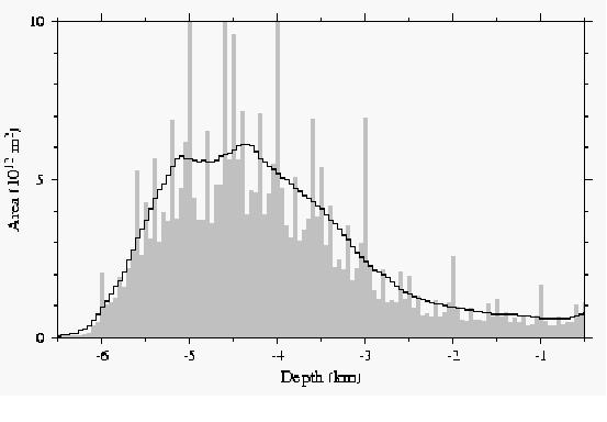
Figure 2.1 Hypsometric curves showing the area of the ocean floor lying between 50 m intervals of depth. Gray boxes (after Smith, 1993) are obtained from the ETOPO-5 grid, while the solid line is obtained from gridded depth estimates derived from altimetry (Smith and Sandwell, 1997). The ETOPO-5 solution illustrates the "terracing" phenomenon — depths near to multiples of 100, 200, and 500 m (evidently contours gridded in DBDB-5) occur more frequently than other values.

DBDB-5 and ETOPO-5 are still in widespread use and have proved quite valuable to the scientific community. Recent developments suggest, however, that the time is ripe for an improved product. A two minute grid of estimated bathymetry based on satellite altimetry between ±72° latitude was released early this year (Smith and Sandwell, 1997), but this is as yet not widely tested and it remains to be seen whether it proves to be useful or accepted.

A.2.2 GEBCO's efforts

The GEBCO SCDB has held informal discussions about producing a gridded data set from the digitised contours in the GEBCO Digital Atlas (GDA) at each of the SCDB's recent meetings. At the meeting in Fredericton in 1994, Ron Macnab presented a new grid for the Arctic Ocean, and the SCDB decided to test various gridding schemes using the recently revised contours available for the area of Sheet 5 - 12 (South Atlantic). An informal working group was organised, which has grown to include Michael Carron, Andrew Goodwillie, Peter Hunter, Meirion Jones, Ron Macnab, Larry Mayer, David Monahan, Bill Rankin, Gary Robinson, Hans-Werner Schenke, and Walter Smith, with Smith serving as chair. The GEBCO Officers encouraged this work at their meeting in 1994 (IOC-IHO/GEBCO Officers-IX/3).

At the 1995 meeting in La Spezia, Hunter, Robinson, and Smith presented gridded versions of the Sheet 5 - 12 area, each prepared with different gridding algorithms. The committee explored the advantages and disadvantages of each. Robinson discussed the strengths and weaknesses of triangulation algorithms and demonstrated the problem of "terracing", which is an artefact of interpolating grids from contour data, but which is not unique to triangulation based algorithms. Smith illustrated what happens when the various solutions are subjected to artificial illumination techniques such as are used in computer visualisations. The group agreed that further exploration of various methods was necessary. The GEBCO Guiding Committee took note of this work at its meeting in 1995 (IOC-IHO/GEBCO-XV/3) and asked the group to develop a short report and recommendations, indicating clearly what can, and what cannot, be achieved in the preparation of a gridded data set. This report is in response to that charge.

When the GEBCO Officers and SCDB met in Honolulu in 1996 there was an informal report of progress by the task group. In addition, Goodwillie reported on his efforts to prepare fine scale grids of the contours drawn by Bob Fisher for the Indian Ocean revisions (Goodwillie, 1996). Hunter, Macnab, Robinson, and Smith met in Southampton in November of 1996 and drew the outline of this report. Meanwhile, Macnab's efforts on the Arctic continued, and led to a paper (Macnab et al., 1997).

When this task group was first convened, the goal was to produce a five arc minute grid to replace the DBDB-5 data. Therefore, some of the examples given in this report refer to that grid spacing. However many of the concepts and results here are scale independent.

Back to top

A.3. Mathematical representations of bathymetry, contours, and grids

A.3.1 Mathematical bathymetry

Computer algorithms for gridding and contouring assume that the bathymetry can be described mathematically. It is supposed that the bathymetry is defined at all points x,y in some region, and at all these points the depth has only one value (there are no vertical or overhanging cliffs), so the depth z can be described as a function z(x,y) . Further assumptions are implicit in contours and in grids.

A.3.2 Mathematical contours continuity

A contour is a set of points x,y at which z has the same value: z(x,y) = c . Contours are only useful when z is a continuous function, so that a contour is a continuous path in the x,y plane and not a set of specks of dust. Since z is single valued, contours of two different values can never cross or touch.

Differentiability

If the contours are not kinked anywhere, so that they have a unique tangent direction at every point, then the following properties hold — z is differentiable, that is, has a unique and finite first partial derivative with respect to x and to y at all points — the gradient (the uphill direction on the surface z(x,y) ) is uniquely defined everywhere and is perpendicular to the local tangent of each contour. If the contour only occasionally has kinks, then the uphill direction can be defined almost everywhere.

Orientation or handedness

Contours with the above properties can be oriented. A direction can be defined so that if one traverses the path of the contour in that direction, the uphill direction on z is always on one's right, or always on one's left. Conventionally, contours are oriented so that uphill lies to one's right. Orientation is useful in graphics applications that fill the areas bounded by contours with colors or patterns.

Completeness and bounding properties.

A contour map is complete if, whenever the value c is contoured somewhere on the map, all the points at which z(x,y) = c have been contoured. That is, if the map is complete and a 4000 m contour appears somewhere on the map, then we can be confident that all locations where z = 4000 have been shown to us. If the map has this property then we can be sure that the regions between the contours are bounded by the contour values — that is, at all points in the space between the 4000 and 4500 m contours z is known to lie between those levels. If the lowest level which appears on the map is 5000 m and we observe that a 5000 m contour encloses a basin deeper than 5000 m, then we do not know the deeper bound on this basin unless we also know what next deeper value would have been contoured.

Note that we use all of these properties, but loosely rather than strictly, when we interpret the morphology of the sea floor from a contour map. A computer algorithm designed to grid contours might use only a limited set of these properties, but might interpret them strictly.

Note also that these properties would not be true of a function with some random noise in it, such as a fractal model of topography, or an estimate derived from some noisy process. Such a function might not be differentiable, or even continuous — it might not be useful to contour such data. Yet such a mathematical model could be useful in other ways if the average value of z averaged in a neighborhood around x,y were accurate. Such is the case, for example, with depth estimates derived in part from satellite altimeter estimates of gravity anomalies — the average properties (at certain scales of averaging) can be very useful, but the estimated value at any point x,y contains enough random noise that contours of the model may not be visually pleasing.

A.3.3 Mathematical grids

Sampling

When one takes measurements of a quantity at regular intervals in time or distance, one is said to have "sampled" the quantity. A two-dimensional sample is conventionally termed a "grid".

Sampling always involves some degree of averaging since the measuring apparatus has a finite resolution, for example the footprint of a sonar transducer. Generally speaking, the resolution of the sampling activity dictates the scale at which the quantity being observed can (or should be) be analysed.

Sampling also introduces uncertainty, since repeated measurements will not in general produce the same value, for example due to variations in the position and orientation of the ship, time dependent refraction effects in the sea water column, and noise in the receiving equipment.

Aliasing

Unless care is taken, the sampling will introduce an error known as "aliasing". An example of aliasing can be seen in any film depicting the accelerations of a vehicle with spoked wheels, such as a stagecoach which departs from a town in a "western" style film. As the stagecoach gains speed, at first it seems that the wheels rotate faster also, but then they appear to slow their rotation, stop, and begin to rotate backward, while at the same time it is clear that the stagecoach is continuing to gain speed. This wrong depiction of the motion of the wheels is an example of aliasing.

The explanation of this phenomenon is due to the film camera taking samples of the scene at fixed intervals of time. As long as the speed of the stagecoach is low enough that the wheels make only a small change in their position between samples, then they will appear to move correctly. However, as the change in the rotation rate of the wheels overtakes the sampling of the film, then the wheels can appear to slow down or turn backwards, whereas they are really accelerating forwards. The fast rotation of the wheels is then said to have been "aliased" into a slow motion (possibly of the wrong sign). Aliasing is thus a consequence of "under-sampling" the quantity being measured or observed.

A bathymetric oriented example is shown in figure 3.1, which represents a cross section through a simple undulating surface. This is sampled regularly in (a) at an interval equal to that of the wavelength of the surface; in (b) at a slightly longer interval; and in (c) at half the wavelength of the undulations. In (a) and (b) the dashed line represents the surface that would be inferred by interpolating between the sampled points; while in (c) and also in (a) it indicates the average value that would be obtained from the sampled points. Two results are evident. First, the actual location of the measurements in (a) influences the value of the average level obtained. Second, sampling the surface at an interval close to its natural wavelength introduces a spurious slope. However, sampling as in (c) reduces both effects.

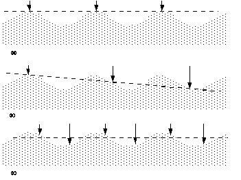
Figure 3.1 Sampling an undulating surface at different frequencies. The dashed line is a linear least squares fit through the samples.

Aliasing can be expressed in mathematical terms using trigonometric functions, since these form a natural basis for operations on equidistantly sampled data. It is shown in elementary texts on time series analysis that if a cosine wave cos (2π f ₁ x ) of frequency f ₁ is sampled at an interval Δ x , it will be aliased into a different cosine wave cos (2π f ₂ x ) of a different frequency | f ₂ | < 1/2Δ x . This is called the Nyquist theorem.

Once we have sampled bathymetry at grid intervals Δ x , the grid cannot represent information at wavelengths shorter than 2Δ x , called the Nyquist wavelength. Furthermore, if the data we are sampling contains information at shorter scales, we must remove that information before taking our samples, otherwise it will become aliased into some erroneous bathymetric feature. Therefore what we want to grid is not the value of depth at the grid point, but rather the average depth in a neighbourhood of size Δ x .

A.3.4 Grids and contours as complementary representations

Contours are the complement or "dual" of grids, in that grids represent a quantity at fixed positions in x and y , whereas contours represent the quantity at fixed (although not necessarily equidistant) intervals in z . Both may be considered as equally valid representations of the quantity and each has its own advantages and disadvantages. Grids are subject to the aliasing problem unless the Δ x is smaller than the scale of features in z , or z has been appropriately averaged before sampling. Contours have a complementary set of difficulties representing the full range of features. Just as grids cannot represent variations on scales smaller than Δ x , so contours cannot represent variations smaller than Δ z , the spacing between successive contours.

A.3.5 Interpolation in contouring of grids

In this report we are concerned with two applications of interpolation. The one we describe in this section is the contouring of grids. In section 5 we will describe methods for estimating values at grid points given source data in the form of contours or soundings or both.

The production of contours from grids is a common operation in computer mapping packages and is carried out at various levels of sophistication. These range from displaying the values at each grid point on a raster display device as colours — giving a filled contour appearance, to the creation of actual contour strings, with gaps left to enable labels to be inserted automatically.

The process of creating a contour string involves navigating or "threading" a path through the rectangle or "cell" formed by four neighbouring grid points (figure 3.2). This can be carried out in a number of different ways, but all involve interpolation in one form or another, and the one most commonly employed is "bi-linear interpolation". Such methods are limited in their ability to produce the "correct" path through the cell when only the four corner points are used. The classic example of this is the "saddle" problem (figure 3.2b), in which the form of the surface within the cell is ambiguous without reference to the context provided by the other surrounding grid points.

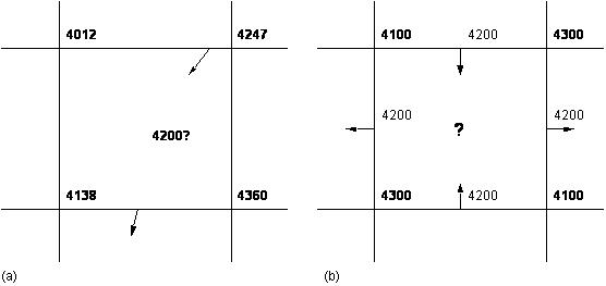
Figure 3.2 Threading contours through a grid cell. In (b) there is potential ambiguity as to the paths to be followed.

Threaded contours often have an angular appearance, especially when using coarse grids, and so these are often smoothed by fitting curves such as splines through them. The danger here is that the additional points may violate the original constraints of the grid, allowing neighbouring contours to cross. This happens because the spline smoothing is done independently of the information in the grid.

It is important to recognise that in producing contours from grids it is the grid resolution that determines the sharpest or smallest feature along a contour.

Back to top

A.4. The representation of bathymetry in the GEBCO contours

A.4.1 Practical realities

The mathematical idealisation that contours are smooth and differentiable, that is, are continuous and not kinked, fails for topographic surfaces that have discontinuities due to ridges and faults at a wide range of scales. The mathematical difficulty may be removed by arguing that our sonar devices have only limited resolution, and so they give us a picture which is necessarily smooth at fine scales. Still, the contouring of faulted or rough surfaces is a theoretical problem.

Contours used in most mapping applications, including GEBCO, are not mathematically ideal for other practical reasons. This is due mainly to cartographic limitations — gaps have to be introduced to enable labels to be inserted and entire swathes of contours have to be left out in areas of high slope to reduce visual "clutter". Conversely, in areas of low relief additional contours are sometimes used, perhaps with "dangling ends", as in GEBCO. These problems are essentially a consequence of using fixed contour levels.

However, a more fundamental reason for the departure from the mathematical ideal is that contours are only an approximation to reality. For example, a 4200 metre contour should not be taken as literally "defining the boundary between depths above/below 4200 metres". Some element of uncertainty must be entertained, since contours are inherently scale dependent — they are generalisations of finer scale detail that cannot be portrayed completely at the given scale.

A.4.2 The GEBCO contours

In GEBCO two methods are used to indicate confidence in contour accuracy — ship tracks and survey boxes, and dashed linework. It is not clear how these should be used to give a quantitative sense of contour accuracy. Furthermore, GEBCO bathymetrists have made use of non-bathymetric information and geological interpretations in drawing contours. The value of this is also difficult to express quantitatively.
An example of geological interpretation is shown in figure 4.1, which shows a section of the Pacific-Antarctic Ridge in the South Pacific. This area has sparse ship track control, and the contours show many features which would not have been generated if a computer gridding and contouring algorithm had been applied to soundings scattered along the survey track lines. For example, in the area around 155° W, 58° S there is a complete absence of survey information, yet the contours have been drawn to show displacement across a fracture zone. Clearly, in this case the contours are meant to illustrate a geologic structure, and while they should not be interpreted as indicating the actual depth, they might correctly indicate the probable direction of slope. Note also that the character and density of the contours south of 60° S is much different from those north of 60° S. The contouring north of 60° S was done by J. Mammerickx, while the contouring south of 60° S was done by L. Johnson and J. R. Vanney. A user of the map who was unaware of this human discontinuity might suppose that there was a genuine change in morphology of the sea bed at 60° S.

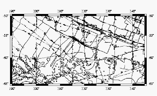
Figure 4.1 The GEBCO contours and ship track control in an area along the Pacific-Antarctic Ridge show the use of geological interpretation to assist contouring.

The GDA contours reflect information at a variety of spatial scales. While a five arc minute grid spacing would probably be sufficient to capture most of the features shown in figure 4.1, there are other areas where this grid size would clearly be insufficient, such as that shown in figure 4.2.

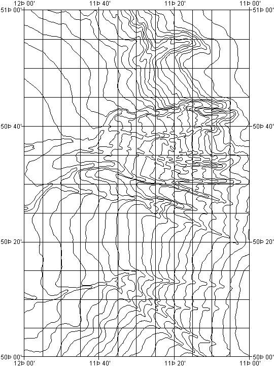
Figure 4.2 Porcupine Sea Bight area in NE Atlantic, showing fine structure in the canyons at the sub arc minute level.

Back to top

A.5. Preparing grids from contours (and possibly other information)

A.5.1 Interpolation algorithms in general

Interpolation is the process of estimating or predicting the value of a quantity at a location where no samples have been taken. In this section we discuss the use of interpolation algorithms to estimate values at grid points from data available as digitised contours, and perhaps other data as well.

Statistical assumptions and statistical methods — kriging and co-kriging.

Most interpolation methods are developed from statistical assumptions. One feature common to all methods is the idea that the data to be interpolated have some spatial correlation — that is, that data values in the neighborhood of a point x,y are of some value in estimating z(x,y) . This assumption must be made, for if it were not so, interpolation would be meaningless and impossible. Another idea implicit in the design of many algorithms is that the sampling of the control data locations has been carried out in a random or near random manner. Of course, this is not the case when the control data are given as digitised contours or as spot values along survey track lines. The density and distribution of control data should be adequate to support accurate interpolation. Nearly all algorithms give suitable and similar results when their control data are adequate. Problems arise when one tries to interpolate values quite far from any control data. It is in such situations that the different behavior of the various algorithms becomes evident.

The simplest methods use local (weighted) averages of the control data, often with a weighting scheme that decreases with distance. These are based on the premise that the closer the point to be estimated lies to a sample point, the more influence the latter should have on the predicted value. Results obtained from such schemes depend on the nature of the weighting function, the size of the neighborhood used, and the distribution of the samples within the neighborhood.

A more sophisticated statistical scheme is one known as "kriging". In this method, one first estimates a statistical model for the spatial correlation among the control data. If the model is a correct one, and certain other assumptions are made (stationarity, etc.), then it can be shown that there is an optimal scheme for choosing the weights and the neighborhood, optimal in the sense that the expected squared error of the interpolation estimate can be minimised. Kriging algorithms yield estimates of z and also estimates of the error in the estimates of z . Proponents of kriging cite its optimal properties to argue that it is the best method, but one should remember that kriging is only as good as the assumptions about statistical properties of z, which it requires.

In a generalisation of kriging known as co-kriging, one makes use of samples of an ancillary variable which shows some covariance with the quantity to be interpolated. For example, one might use gravity anomaly data obtained from satellite altimetry as a guide to interpolation of bathymetry. In co-kriging, one would first need to make assumptions about the statistical properties of both data types, then estimate the covariance function for the data, and then proceed to estimate the interpolated depths using both data types. The depth estimation scheme using altimetry of Smith and Sandwell (1994; 1997) is analogous to co-kriging in some respects. Smith and Sandwell use a "transfer function" which is based on theoretically expected correlations between bathymetry and gravity. A transfer function is essentially the Fourier transform of a covariance function. They also assume that covariance between gravity and bathymetry, if it is present at all, will be seen only in bandpass filtered residuals of those quantities. Such filtering ensures that the data will not violate the necessary assumptions, but it also limits the precision of the results.

Global versus local schemes — "high-order" methods

A "global" interpolation scheme is one in which some part of the process is derived from an operation on the entire input data set taken as a whole. The simplest such operation would be fitting of a trend surface to the entire data set by regression. Kriging is also a global method, in principle, in that the global (sum of the entire) squared error expected in the estimate is minimised. The data are used globally to estimate the covariance function. However, after one has obtained this function, its structure usually shows that an average in a local neighborhood is sufficient, so that the computation proceeds locally after the covariance estimation.

Another kind of "global" scheme is one in which the goal is to obtain "smooth" solutions. By smooth, one means that an interpolating function is found which has global continuity of one or more of its derivatives — that is, it has no sharp kinks or edges. The most common scheme of this kind is known as "minimum curvature" or "minimum tension", and finds an interpolant which has continuous second derivatives and minimises the global (integral of the entire) squared curvature (estimated by the surface Laplacian) of z(x,y) . Although this global property is used to design the method, the solution can be found by iteration of a local weighted averaging operator (Briggs, 1974; Smith and Wessel, 1990). The continuity of the derivatives is a useful property for gridding data which will be contoured or imaged using artificial illumination — the contours won't have kinks and the highlights and shadows will have a smooth, natural appearance.

In contrast, since it is computationally more efficient to build the local interpolation estimate only from values in the neighbourhood of the estimated point, some "local" schemes operate on data only locally. This is justified when the correlation in the data approaches zero outside of some neighbourhood size. One simple method is to use a fixed radius or other geometric threshold. However, this is subject to variations in the data density. A solution is to vary the search distance "on the fly" to ensure that sufficient points are obtained, and this method is employed successfully in many interpolation software packages.

An alternative approach is to organise the data spatially into a network, or "triangulation". This automatically constrains the interpolation process so that only the three points surrounding the point to be estimated are used, with the estimate being derived via linear interpolation over the triangle formed by these points. The network of planar triangular facets so obtained does not have continuous derivatives, however. A refinement is to use a curved surface fitted through the three points using estimates of the first order derivatives — these can be found by using the immediate neighbours of each point. The success of triangulation based interpolation relies on a satisfactory data distribution. Ideally, each triplet of points should be reasonably spatially correlated, so that it is valid to represent the region between them by a plane or other simple function. Contours provide a particular challenge in this respect, as discussed in following section.

Interpolation inevitably introduces a degree of uncertainty, in addition to that inherent in the samples that are used in the averaging process. Kriging, which has its origins in geostatistical theory, has the benefit of producing a quantifiable estimate of the interpolation error at each point. Interpolation schemes which yield continuity of derivatives are called "higher-order", in contrast to those which yield continuity only of the interpolated quantity.

A.5.2 Behaviour of interpolation algorithms applied to digitised contour input

With the exception of some triangulation based techniques, most interpolation methods do not use the information that is present in contours, i.e. the fact that they contain information about the local slope. Worst still, some even ignore the bounds constraints of the ideal contours. Higher order effects, such as overshoot and undershoot are also a problem with many algorithms, especially those that fit high order curves or surfaces through data points, such as splines. This problem is exacerbated by trying to fit the surface exactly to the data. Perhaps the worst problem occurs in data "voids".

An example is shown schematically in Figure 5.1 below. Shown are some points, and two interpolations through them. The points shown are meant to illustrate what happens when digitised contours are interpolated by low order and high order schemes. The points represent values at 0, 100, 200, 500 m, and then every 500 m to 5000 m, in a profile across a continental shelf, slope, and abyssal plain. The low order scheme fits planar surfaces between the contours, which appear as straight line segments in this cross-section (solid lines). The higher order scheme produces a curved surface, with a cross-section as shown by the dashed line. The abyssal plain and continental shelf are data "voids" as far as these algorithms are concerned — the algorithms do not "feel" any constraint in these areas — they do not "know" that the depths are bounded by the contours that surround these regions. The low order scheme honours the bounds of the contours, but only because it cannot do anything else — it cannot make smooth transitions between the constraints, but only planar facets joined by sharp kinks.

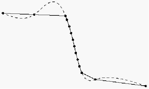
Figure 5.1 Hypothetical profile across a continental shelf, slope, and abyssal plain, showing a "high-order" interpolation algorithm violating bounds constraints implied by contours (dots).

The minimum curvature spline algorithm used to prepare DBDB-5 is of the high order class, and can have the overshoots illustrated above (Smith and Wessel, 1990). The "surface" program in the GMT graphics package (Wessel and Smith, 1991) is a generalisation of the minimum curvature algorithm in which "tension" can be added to the solution to suppress the overshoots shown in Figure 5.1. A later generalisation in an updated version (Wessel and Smith, 1995) has an option to add bounds constraints, and is intended for situations like the gridding of contours.

A low order method applied to a triangulation of digitised contours does achieve an honouring of most of the constraints implied by the mathematical view of contours. Each triangle will have at least two of its three vertices lying along a contour, and since the interpolating function is planar, the function will honour the bounds and it will have a gradient in the direction perpendicular to one of the contours. However, when two contours follow one another in a nearly parallel fashion, triangulation has a tendency to generate different gradients in alternating triangles. The result can look very peculiar when subjected to artificial illumination in visualisation techniques. An example is shown below, for an area near South America in Sheet 5.12. Note the gradient at the continental shelf break.

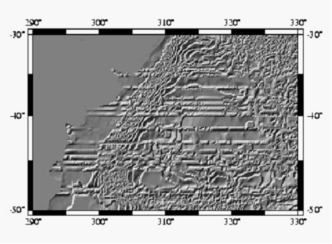
Figure 5.2 Artificial illumination from the northwest of a (low order) triangulated interpolation of the contours of Sheet 5.12 (revised). From one of the examples prepared by Robinson for the SCDB in La Spezia in 1995.

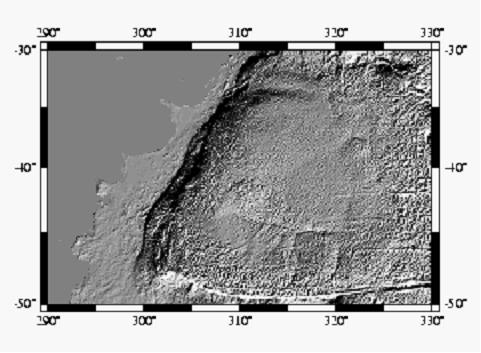
Figure 5.3 Same as 5.2, but from the altimeter guided estimate of Smith and Sandwell (1997).

Tradeoffs and problems

Low order methods may honour the bounds constraints of contours, but at the expense of unsmooth derivatives. High order methods offer smooth derivatives, but may violate the bounds constraints. In principle, the new version of GMT's "surface" should be able to honour bounds while offering a high order technique, but this has not been tried yet.

The terracing problem was illustrated earlier. The problem is made worse when the contours are digitised with fine detail, so that the distance between samples along the contour path is much smaller than the distance between contours. Low order triangulation may be more subject to terracing than a high order scheme.

Kriging includes the nice feature of estimating the error in the estimated solution. However, estimation of an appropriate correlation function from the data is very difficult when the input constraints are digitised contours, because all the differences between points are quantised to be multiples of the contour interval, giving biased results.

A.5.3 Practicalities of using the GEBCO contours

As discussed in the introduction, initial experiments with existing gridding techniques to create five arc minute grids using the contours from the GDA have identified a number of issues that must be addressed. Most of these centre on the nature of the GEBCO contours. More specifically, in many geographical areas the GEBCO contours do not provide a sufficiently uniform coverage that is essential for optimal interpolation onto a regular grid (of whatever resolution). Figures 5.4 and 5.5 may be used to illustrate this problem. These show areas with sparse contour coverage due to the relatively flat nature of the continental shelf and abyssal plains, respectively. In both cases we may say that these regions are grossly under sampled, particularly given the amount of detail that appears in the surrounding contours. However, in the case of abyssal plains a mitigating factor is that we know that they are in reality extremely flat, and we can use this information in the gridding process.

A.5.4 Grid resolution

The question of grid resolution is quite difficult to resolve. On the one hand the information in the contours is highly detailed and would require a grid of the order of one arc minute or less to reproduce (figure 4.2). On the other hand, at the global level the mean spacing between contours points to the use of a much larger spacing, perhaps of the order of five to eight arc minutes. Unless we resort to variable grids (c.f. DBDB-V), we must chose a compromise value. Given the relative cheapness of computer storage these days, opting for a small grid spacing — and consequently a high data volume — is not a serious problem. However, this must be balanced by not giving the impression that small spacing = high resolution, i.e. "more accurate". This latter point should perhaps be addressed by the quality information that accompanies the gridded data set.

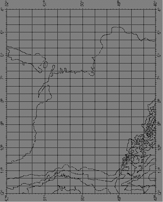
Figure 5.4 SW Approaches to UK, showing extent of continental shelf and detailed contours at the shelf slope.

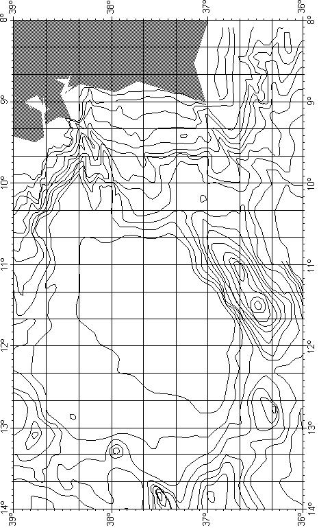
Figure 5.5 Non-uniform distribution of contours — Off the Iberian peninsula, the featureless Tagus abyssal plain in the centre of the figure is devoid of contours but is surrounded by areas of pronounced bathymetric variability.

A.5.5 Avoiding aliasing

There are basically two ways of avoiding aliasing problems when gridding, particularly where contours are the primary source of data.

The first is to average the source data using a simple box averaging process (the size of the box should be of the same size as the target grid cell size, but may be slightly smaller). This results in one data point per box, with the value and position of the point being determined by the geometrically weighted average of all the points within the box (figure 5.6). This has little effect on data in sparse regions (especially boxes without data points!), but does reduce the high frequency variation in detailed areas. The disadvantage of this technique is that because the point density of contour based data is biased towards the more detailed stretches, undue weighting may be given to those contours. This can lead to the terracing effect discussed earlier. To minimise this, the data points should also be weighted by the distances to their neighbouring points along the same contour.

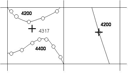
Figure 5.6 Using box averaging to reduce aliasing effects prior to gridding. Note that single points are unaffected. Key: — = contour; o = digitised point; + = "average" point.

The second method involves generating a very fine grid from all of the data, perhaps on a piecewise basis to cope with variations in data density. This is then averaged to give the final grid. The main advantage of this method is that it automatically yields statistics such as standard deviation and extreme values of the depth. This method is particularly suited to triangulation based interpolation techniques.

Back to top

A.6. References

Briggs, I. C. , Machine contouring using minimum curvature, Geophysics, 39, 39-48, 1974 .

Goodwillie, A. M., 1996 . Producing Gridded Databases Directly From Contour Maps. University of California, San Diego, Scripps Institution of Oceanography, La Jolla, CA. SIO Reference Series No. 96-17, 33p.

Macnab, R., G. Oakey, and D. Vardy , An improved portrayal of the floor of the Arctic ocean based on a grid derived from GEBCO bathymetric contours, submitted to Int'l. Hydrogr. Rev., 1997 .

Sandwell, D. T., and W. H. F. Smith , Marine gravity anomaly from Geosat and ERS-1 satellite altimetry, J. Geophys. Res., 102, 10,039-10,054, 1997 .

Smith, W. H. F. , On the accuracy of digital bathymetric data, J. Geophys. Res., 98, 9591-9603, 1993 .

Smith, W. H. F., and D. T. Sandwell , Bathymetric prediction from dense satellite altimetry and sparse shipboard bathymetry, J. Geophys. Res., 99, 21,803-21,824, 1994 .

Smith, W. H. F., and D. T. Sandwell , Global seafloor topography from satellite altimetry and ship depth soundings, submitted to Science, 1997 .

Smith, W. H. F., and P. Wessel , Gridding with continuous curvature splines in tension, Geophysics, 55, 293-305, 1990 .

World Data Center A for Marine Geology and Geophysics , ETOPO-5 bathymetry/topography data, Data announcement 88-MGG-02, Nat'l. Oceanic and Atmos. Admin., US Dept. Commer., Boulder, Colo., 1988 .

Wessel, P., and W. H. F. Smith , Free software helps map, display data, EOS Trans. Am. Geophys. U., 72, 441, 446, 1991 .

Wessel, P., and W. H. F. Smith , New version of the Generic Mapping Tools released, EOS Trans. Amer. Geophys. Un., 76, 329, 1995 , with electronic supplement on the World Wide Web at http://www.agu.org/eos_elec/95154e.html .

Back to top

APPENDIX B — Version 2.0 of the GEBCO One Minute Grid

The GEBCO One Minute Grid was originally released in 2003 as part of the Centenary Edition of the GEBCO Digital Atlas (GDA). It is largely based on the bathymetric contours contained within the GDA with additional data used to help constrain the grid in some areas. You can find out more about the development of the grid from the documentation which accompanies the data set (GridOne.pdf).

Version 2.0 of the GEBCO One Minute Grid was released in November 2008 and includes version 2.23 of the International Bathymetric Chart of the Arctic Ocean (IBCAO) and updated bathymetry for some shallow water areas around India and Pakistan, the Korean Peninsula and South Africa.

Included in version 2.0 of the GEBCO One Minute Grid

• Version 2.23 of the International Bathymetric Chart of the Arctic Ocean
• Shallow water bathymetry updates for —
  • waters around India and Pakistan
  • waters around the Korean Peninsula
  • waters around South Africa
• Updates for some reported bug fixes in version 1.0 of the GEBCO One Minute Grid

Version 2.23 of the International Bathymetric Chart of the Arctic Ocean (IBCAO)

Authors — Martin Jakobsson ¹ , Ron Macnab ² , Larry Mayer ³ , Robert Anderson ⁴ , Margo Edwards ⁵ , Jörn Hatzky ⁶ , Hans Werner Schenke ⁶ and Paul Johnson ^6
1 Department of Geology and Geochemistry, Stockholm University, Sweden
² Canadian Polar Commission, Nova Scotia, Canda
³ Center for Coastal and Ocean Mapping, University of New Hampshire, NH, USA
⁴ SAIC-Science Applications International Cooperation, WA, USA
⁵ Hawaii Institute of Geophysics and Planetology, University of Hawaii, Honolulu, HI, USA
⁶ Alfred Wegener Institute, Brmerhaven, Germany

Data set limits — north of 64° N to 90° N; 180° W to 180° E

Citation — Jakobsson, M., Macnab, R., Mayer, M., Anderson, R., Edwards, M., Hatzky, J., Schenke, H-W., and Johnson, P., 2008 , An improved bathymetric portrayal of the Arctic Ocean: Implications for ocean modeling and geological, geophysical and oceanographic analyses, v. 35, L07602, Geophysical Research Letters, doi:10.1029/2008GL033520

The IBCAO was first released in 2000. Since then there have been a number of multibeam surveys in the Arctic Ocean region which have significantly improved our knowledge of the shape of the seafloor in this region. The IBCAO team felt this warranted an update to the IBCAO data set and version 2.23 of the IBCAO was released in March 2008.

Further details about the IBCAO data set along with grids and maps for downloading can be found at: http://www.ibcao.org/ .

Shallow water bathymetry data updates

GEBCO has traditionally depicted the bathymetry of the deeper water areas of the world's oceans, i.e. at depths of 200 m and deeper. In order to more adequately represent the shape of the ocean floor in all areas, and to serve a wide range of users, the GEBCO community has recognised the importance of improving the GEBCO One Minute Grid in shallow water areas.

The bathymetry data held collectively by International Hydrographic Organization (IHO) Member States in the Electronic Navigation Chart (ENC) system was recognised as a valuable source of data which could be used to significantly improve the existing and future GEBCO grids in shallow water regions.

Extracting bathymetry data from ENCs

A software application was developed to simplify the extraction of data from ENC files (usage bands two and three). This software package was supplied to IHO Member States on request. This work was co-ordinated by the International Hydrographic Bureau (IHB).

Many Hydrographic Offices have already contributed shallow water bathymetry data. Data for three regions have so far been used to update the GEBCO One Minute Grid. This work is described below.

Updating the GEBCO One Minute Grid

Sounding point data extracted from ENCs for the areas around India and Pakistan, the Korean Peninsula and South Africa has been used to update the GEBCO One Minute Grid and have been released as part of version 2.0 of this data set.

Work on the incorporation of shallow water bathymetry data into the GEBCO One Minute Grid was carried out at the British Oceanographic Data Centre (BODC). For further information contact Pauline Weatherall ( paw@bodc.ac.uk ).

The general method used to update the grid in shallow water regions is described below. Further information about the data provided and the generation of the grid for each of these separate areas is given at the end of this document.

Data source — soundings extracted from ENCs

For each region, sounding points were provided from a number of overlapping ENC data sets. An attempt has been made to edit data from overlap regions. Only those ENC sounding points shallower than 300 m were used in the gridding work.

The ENC data are to chart datum — no attempt has been made to adjust the data for the state of the tide.

Data source — original GEBCO One Minute Grid

The aim of this work is to update the existing GEBCO grid in shallow water regions, therefore the ENC sounding point data were combined with the original source data used to generate the GEBCO One Minute Grid, i.e. bathymetric contours from the GEBCO Digital Atlas, additional control used to constrain the grid — World Vector Shoreline and land elevation data from the Global Land One-km Base Elevation (GLOBE) project data set.

Harmonising the data sets

A Geographic Information System (GIS) was used to visualise the relationship between the original grid source data sets and the ENC sounding points. In some areas it was necessary to edit the GEBCO bathymetric contours to harmonise the data sets. The ENC sounding points, GEBCO bathymetric contours, additional grid control data, coastline and land elevation data were then combined into one ASCII XYZ file.

Gridding work

The gridding work was done using routines from the Generic Mapping Tools (GMT) suite of software. The data were first filtered using the 'blockmedian' routine. The gridding was done using the 'surface' routine.

The grids were then checked for any errors or grid artefacts and the gridding process was repeated if necessary.

More detailed information about the generation of the grids for each area follows below.

Please note that although the grid has been improved in shallow water regions the data set is not to be used for navigation or any purpose relating to safety at sea.

Improving the GEBCO One Minute Grid in the area around India and Pakistan

Geographic area — Coastal regions shallower than 300 m between 62° 12' E and 87° E
ENC data set provider — National Hydrographic Office, India

The data set supplied by the National Hydrographic Office, India consists of 44 separate ENC data files.

Only those ENC sounding points shallower than 300 m were used in the gridding work, the resulting data file contains 27,113 points. The image below shows the coverage of the ENC sounding points used to generate the grid.

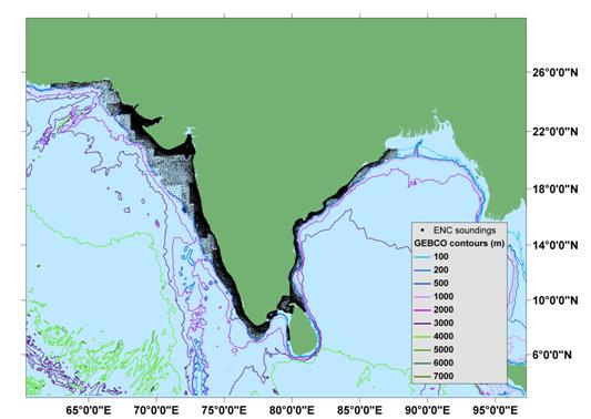
Distribution of ENC sounding points used in the gridding work

The histogram below shows the number of sounding points from the ENC data set per 50 m depth interval used to update the GEBCO One Minute Grid.

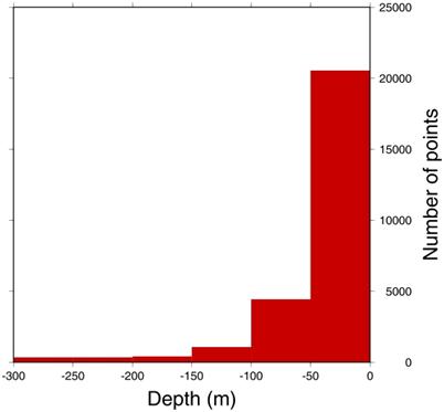
A Geographic Information System (GIS) was used to visualise the relationship between the original grid source data — i.e. bathymetric contours from the GEBCO Digital Atlas and the ENC sounding points. In some areas it was necessary to edit the GEBCO bathymetric contours to harmonise the data sets. The ENC sounding points, GEBCO bathymetric contours, additional grid control data, coastline and land elevation data were then combined into one ASCII XYZ file.

The gridding work was done using Generic Mapping Tools (GMT) software routines.

Improving the GEBCO One Minute Grid in the area around the Korean Peninsula

Geographic area — coastal areas shallower than 300 m between 123° 56' E and 132° E
Data provider — National Oceanographic Research Institute (NORI), Republic of Korea

The data set supplied by NORI consists of bathymetric soundings, bathymetric contours, coastline data and quality of data information polygons. The bathymetric sounding point data set were used for the gridding work. The data are taken from 82 separate ENC data files.

Only those sounding points shallower than 300 m have been included for the gridding work. The resulting data file used for gridding contains 96,061 points.

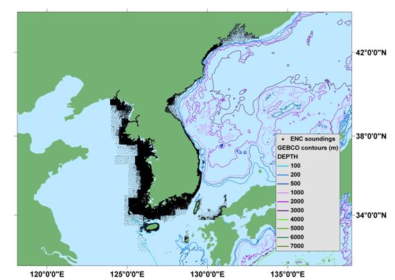
Distribution of ENC sounding points used in the gridding work

The histogram below shows the number of sounding points from the ENC data set per 50 m depth interval used for gridding.

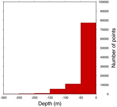
A Geographic Information System (GIS) was used to visualise the relationship between the original grid source data — i.e. bathymetric contours from the GEBCO Digital Atlas and the ENC sounding points. In some areas it was necessary to edit the GEBCO bathymetric contours to harmonise the data sets. The ENC sounding points, GEBCO bathymetric contours, additional grid control data, coastline and land elevation data were then combined into one ASCII XYZ file.

The gridding work was done using routines from the Generic Mapping Tools (GMT) system.

Improving the GEBCO One Minute Grid in the area around South Africa

Geographic area — coastal areas shallower than 300 m between 16° 20' E and 32° 54' E
Data provider — South African Hydrographic Office

The data set supplied by the South African Hydrographic Office consists of bathymetric soundings, bathymetric contours, coastline data and quality of data information polygons. The bathymetric sounding point data set were used for the gridding work. The data are taken from 23 separate ENC data files.

Only those ENC sounding points shallower than 300 m were used in the gridding work, the resulting data file contains 9,622 points. The image below shows the coverage of the ENC sounding points used to generate the grid.

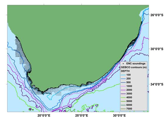
Distribution of ENC sounding points used in the gridding work

The histogram below shows the number of sounding points from the ENC data set per 50 m depth interval used for gridding.

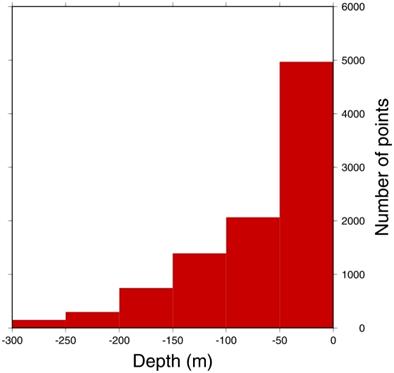
A Geographic Information System (GIS) was used to visualise the relationship between the original grid source data — i.e. bathymetric contours from the GEBCO Digital Atlas and the ENC sounding points. In some areas it was necessary to edit the GEBCO bathymetric contours to harmonise the data sets. The ENC sounding points, GEBCO bathymetric contours, additional grid control data, coastline and land elevation data were then combined into one ASCII XYZ file.

The gridding work was done using Generic Mapping Tools (GMT) routines.

Updates for reported bugs in version 1.0 of the GEBCO One Minute Grid

Version 2.0 of the GEBCO One Minute Grid includes updates for reported bugs in the Hudson Bay area and off the west coast of Africa.

A list of reported bugs in the GEBCO One Minute Grid can be found on the following web site — http://www.bodc.ac.uk/help_and_hints/errata/gebco.html

Back to top